
Confidence Intervals and Sample Size, Worked Through
Where the margin of error comes from, when to use t instead of z, why the Wilson interval beats Wald for proportions, and how 385 became the default survey size.
By Redbison Dev · · Updated · 9 min read
A sample gives you an estimate: 31% of customers would recommend you, the average part is 12.14 mm long. The question that follows is always "how sure are you?" A confidence interval answers it after the data are in, and a sample size calculation answers it before you start. Both rest on the same small formula, and this guide works through it with the Confidence Interval Calculator and the Sample Size Calculator so every number can be checked.
The one formula behind both tools
Almost every interval in introductory statistics has the same shape:
estimate ± critical value x standard error
The standard error is how much the estimate would wobble from sample to sample. For a mean it is s / √n; for a proportion it is √(p(1 - p) / n). The critical value sets how many standard errors wide the interval must be for the confidence level you want: 1.96 for 95% with the normal distribution, more with the t distribution. Their product is the margin of error.
Turn the formula around and you get sample size. If you decide in advance that the margin must be at most E, then E = z x √(p(1 - p) / n), and solving for n gives n = z² p(1 - p) / E². Everything in this guide is a variation on those two lines.
Intervals for a mean: t or z?
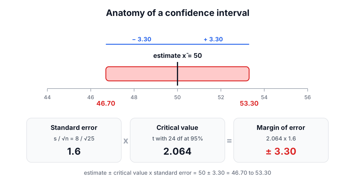
Suppose 25 measurements have mean 50 and standard deviation 8. The standard error is 8 / √25 = 1.6.
If you somehow knew the population standard deviation was 8, you would use the normal critical value 1.96 and get 50 ± 3.14. But you almost never know σ; you estimated it from the same 25 values, and that estimate has its own error. William Gosset, writing as "Student" in 1908 while working on small samples at the Guinness brewery, worked out the distribution that accounts for this. The t distribution looks like the normal but with heavier tails, and how heavy depends on the degrees of freedom, n - 1.
With 24 degrees of freedom the 95% critical value is 2.064, so the interval is 50 ± 3.30, from 46.70 to 53.30. The difference from z grows quickly as samples shrink:
| Sample size | Degrees of freedom | 95% t critical value |
|---|---|---|
| 2 | 1 | 12.706 |
| 5 | 4 | 2.776 |
| 11 | 10 | 2.228 |
| 31 | 30 | 2.042 |
| very large | very large | 1.960 |
The practical rule is simple: if the standard deviation came from your sample, use t. It is never wrong, and for large samples it gives the same answer as z anyway. Reserve z for the rare case where σ is genuinely known, for example from a long-running, stable manufacturing process.
The t interval also assumes the sample mean is close to normally distributed. With 30 or more values the central limit theorem usually takes care of that. With 8 values, glance at the data first: one wild value or a strongly skewed shape makes the interval less trustworthy.
Intervals for a proportion: why Wilson beats Wald
The interval most textbooks teach for a proportion is the Wald interval, p̂ ± z√(p̂(1 - p̂) / n). It is the general formula with the sample proportion plugged into the standard error. It is easy, and it is unreliable.
Two problems stand out. First, at the edges it breaks completely. With 0 successes out of 30, p̂ = 0, the standard error is 0 and the Wald interval is "0% to 0%", a claim of perfect certainty from 30 observations. Second, even away from the edges its actual coverage is often well below the stated 95%. Lawrence Brown, Tony Cai and Anirban DasGupta showed in a 2001 paper that the coverage swings erratically as n and p change, and can fall well short of the nominal level even with samples in the hundreds when p is near 0 or 1.
The Wilson score interval, published by Edwin Bidwell Wilson in 1927, fixes both. Instead of plugging p̂ into the standard error, it asks which values of the true proportion would not be rejected by a test given the data, and solves for them. The result:
- centre = (p̂ + z²/2n) / (1 + z²/n)
- half-width = z √(p̂(1 - p̂)/n + z²/4n²) / (1 + z²/n)
The centre is pulled slightly toward 50%, the interval is asymmetric near the edges (as it should be, since a proportion cannot go below 0), and its coverage stays close to 95%.
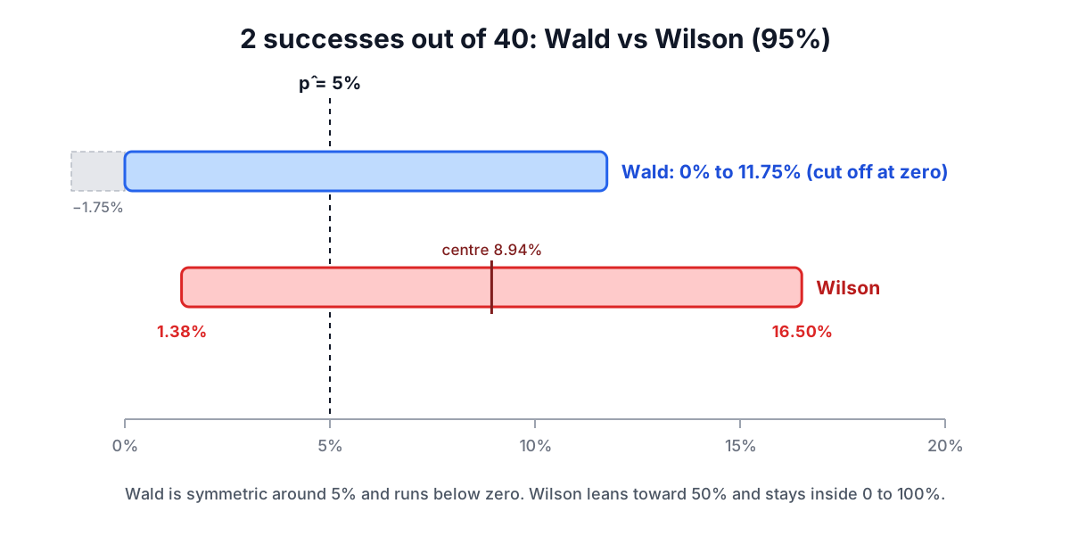
For 2 successes out of 40 (5%), Wald gives -1.75% to 11.75%, truncated to 0% to 11.75%. Wilson gives 1.38% to 16.50%. For 0 out of 30, Wilson gives 0% to 11.35% rather than a zero-width interval. For 81 out of 263, a well-behaved case, the two nearly agree: Wald 25.22% to 36.38%, Wilson 25.53% to 36.62%. Those last figures match Robert Newcombe's 1998 comparison of interval methods, which is one of the checks in the calculator's tests.
The calculator shows both and flags the Wald interval whenever there are fewer than 10 successes or 10 failures. Report Wilson.
What "95% confident" means
A 95% confidence interval comes from a procedure that, if you repeated the whole study many times, would capture the true value in 95% of the repetitions. Any single interval either contains the truth or does not; the 95% describes the method's track record.
Two consequences are worth remembering. First, a confidence interval only accounts for random sampling error. If your survey reached only people who answer phone calls from unknown numbers, the interval says nothing about that bias. Second, the width shrinks with the square root of n, so precision gets expensive: to halve the margin of error you need four times the data.
How many responses do you need?
The survey version of the formula is Cochran's:
n₀ = z² p(1 - p) / E²
At 95% confidence (z = 1.959964), a margin of ±5% (E = 0.05) and p = 0.5:
n₀ = 3.8415 x 0.25 / 0.0025 = 384.15, which rounds up to 385.
That is where the ubiquitous 385 comes from. The p = 0.5 is deliberate: p(1 - p) is largest at 50%, so using it gives the biggest, safest sample. If earlier research says the answer is about 20%, p(1 - p) = 0.16 and n falls to 246, but if the true value turns out to be nearer 50% you will miss your margin.
Some standard results for a large population:
| Confidence | ±10% | ±5% | ±3% | ±1% |
|---|---|---|---|---|
| 90% | 68 | 271 | 752 | 6,764 |
| 95% | 97 | 385 | 1,068 | 9,604 |
| 99% | 166 | 664 | 1,844 | 16,588 |
Small populations
Cochran's formula assumes sampling from an effectively infinite population. When the population is small, each response removes a meaningful share of the uncertainty, and the finite population correction applies:
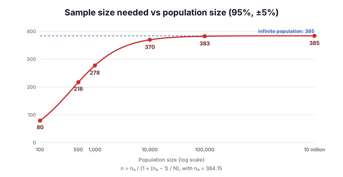
n = n₀ / (1 + (n₀ - 1) / N)
For a company of 500 employees, 385 becomes 218. For 1,000 it becomes 278, and for 100 it becomes 80. For a city of a million it is 384, essentially unchanged. This is why a national poll of about 1,000 people has the same ±3.1% margin whether the country has 5 million or 300 million people: once the population is much bigger than the sample, its size stops mattering.
Means instead of percentages
To estimate an average within ±E you need a guess at the standard deviation: n = (zσ / E)². If a pilot study suggests σ = 15 and you want the mean within ±2 at 95%, n = (1.96 x 15 / 2)² = 216.08, so 217. The answer is only as good as the σ guess, so round up generously.
From responses to invitations
The formula gives completed responses. If you expect 25% of invitations to come back, divide by 0.25: 385 responses means inviting 1,540 people. Low response rates also raise the risk that responders differ from non-responders, which no sample size can fix.
Judgment calls the formulas leave to you
- Subgroups need their own sample. If you want ±5% for each of four regions, you need about 385 per region.
- Comparing groups is a different calculation. Detecting a difference between two conversion rates needs a power analysis that also depends on the smallest difference worth detecting. The formulas here size a single estimate.
- Complex designs need a design effect. Cluster sampling (whole schools, whole households) gives less information per person, so multiply the sample by a design effect, often between 1.5 and 2.
- Pick the margin by the decision. If the result will only change what you do when it moves by 10 points, a ±3% survey is wasted effort.
Get those right and the arithmetic is the easy part, which is exactly what the calculators are for. For the descriptive statistics that feed these formulas, including why the sample standard deviation divides by n - 1, see the descriptive statistics guide.
Frequently asked questions
Why is the standard survey sample size 385?
The 385 comes from Cochran's formula, n₀ = z² p(1 - p) / E², at 95% confidence (z = 1.959964), a ±5% margin and p = 0.5. That gives 3.8415 x 0.25 / 0.0025 = 384.15, which rounds up to 385. Using p = 0.5 is deliberate, because p(1 - p) is largest at 50%, giving the biggest, safest sample.
What is the finite population correction for sample size?
The finite population correction reduces the required sample when the population is small: n = n₀ / (1 + (n₀ - 1) / N). At 95% confidence and ±5%, 385 becomes 218 for a population of 500, 278 for 1,000 and 80 for 100. For a city of a million it is 384, so once the population is far bigger than the sample, its size stops mattering.
How do I calculate sample size to estimate a mean?
To estimate a mean within ±E, use n = (zσ / E)², which needs a guess at the standard deviation σ. If a pilot study suggests σ = 15 and you want the mean within ±2 at 95% confidence, n = (1.96 x 15 / 2)² = 216.08, so you need 217. The answer is only as good as the σ guess, so round up generously.
How many survey invitations should I send?
Sample size formulas give completed responses, so divide by the expected response rate to get invitations. If you need 385 responses and expect 25% of invitations to come back, invite 1,540 people. Low response rates also raise the risk that responders differ from non-responders, which no sample size can fix.
How much more data do I need to halve the margin of error?
You need four times the data to halve the margin of error, because the width of a confidence interval shrinks with the square root of the sample size. At 95% confidence and p = 0.5, a ±5% margin needs 385 responses while ±3% needs 1,068 and ±1% needs 9,604, so precision gets expensive quickly.
Sources and further reading
- The Probable Error of a Mean, Biometrika. Gosset's 1908 paper introducing the t distribution.
- Interval Estimation for a Binomial Proportion, Statistical Science. Brown, Cai and DasGupta, 2001.
- Probable Inference, the Law of Succession, and Statistical Inference, Journal of the American Statistical Association. Wilson, 1927.
- Two-sided confidence intervals for the single proportion: comparison of seven methods, Statistics in Medicine. Newcombe, 1998, abstract on PubMed.
- Approximate is Better than Exact for Interval Estimation of Binomial Proportions, The American Statistician. Agresti and Coull, 1998.
- Sampling Techniques, 3rd Edition, Wiley. Cochran's sample size formulas.
- Margin of Sampling Error/Credibility Interval, American Association for Public Opinion Research. How pollsters report the margin of error.
Open the Confidence Interval Calculator
More Statistics Calculators
Every tool in the Statistics Calculators section, free and in your browser.
- Standard Deviation Calculator
- Mean, Median and Mode Calculator
- Z-Score Calculator
- Confidence Interval Calculator
- Sample Size Calculator
- Permutation and Combination Calculator
- Probability Calculator
- Linear Regression Calculator
- T-Test Calculator
- P-Value Calculator
- Chi-Square Calculator
- Normal Distribution Calculator
- One-Way ANOVA Calculator