
Probability Rules, Permutations and Combinations
Counting outcomes with nPr and nCr, the addition and multiplication rules, conditional probability, the at-least-one trick and when the binomial model applies.
By Redbison Dev · · Updated · 9 min read
Most probability problems in school, in games and in everyday risk come down to two skills: counting the outcomes correctly, and combining the probabilities of events with the right rule. This guide covers both, with numbers you can check in the Permutation and Combination Calculator and the Probability Calculator.
Counting: does order matter, and can items repeat?
Every counting question answers two yes-or-no questions. Does the order of the chosen items matter? Can the same item be chosen more than once? The four answers give four formulas.
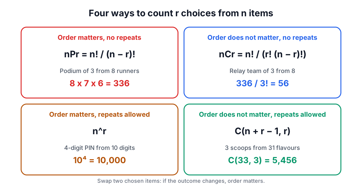
Ordered, no repetition: permutations. Eight runners, three podium places. Any of 8 can win, then any of the remaining 7 can come second, then any of 6 can come third: 8 x 7 x 6 = 336. In factorial form, nPr = n! / (n - r)! = 8! / 5!.
Unordered, no repetition: combinations. Choose 3 of the 8 runners for a relay team where positions do not matter. Each team of three was counted 3! = 6 times in the 336 podiums (ABC, ACB, BAC, BCA, CAB, CBA), so there are 336 / 6 = 56 teams. In general nCr = n! / (r! (n - r)!). A five-card poker hand is the classic example: 52C5 = 2,598,960 possible hands, because being dealt the ace first or last makes no difference.
Ordered, with repetition. A 4-digit PIN has 10 choices for each of 4 positions: 10⁴ = 10,000. If the digits had to be different, it would be 10P4 = 5,040.
Unordered, with repetition. Three scoops in a cup from 31 flavours, repeats allowed, order irrelevant. The trick, known as stars and bars, is to think of the cup as 3 stars separated into 31 flavour bins by 30 bars. Choosing where the 3 stars go among 33 positions gives C(33, 3) = 5,456.
A quick test for order: swap two of the chosen items. If the outcome is different (first and second place swapped), order matters. If it is the same (two people on a committee swapped), it does not.
Why exact arithmetic matters
Factorials explode. 20! is already 2.4 x 10¹⁸, beyond the range where ordinary floating-point numbers keep every digit, and 171! overflows a standard double entirely. Computing nCr as n! divided by two other factorials in floating point therefore loses precision long before the answer itself gets large. The calculator uses arbitrary-precision integers and divides at every step of the product, so 100C50 comes out as the exact 30-digit integer 100,891,344,545,564,193,334,812,497,256.
From counts to probabilities
When all outcomes are equally likely, probability is favourable outcomes over total outcomes. The chance of being dealt a specific five-card hand is 1 in 2,598,960. A Powerball ticket must match 5 white balls from 69 (69C5 = 11,238,513) and 1 red ball from 26, so the jackpot odds are 1 in 11,238,513 x 26 = 292,201,338.
The three rules for combining events
Once you have probabilities for single events, three rules combine them.
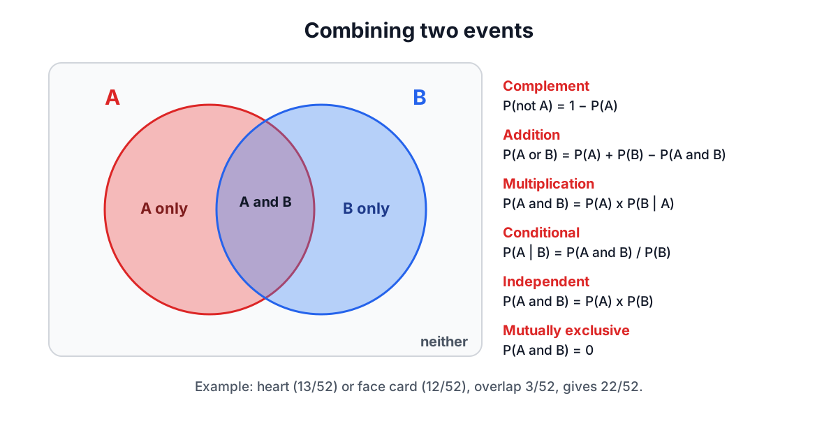
Complement. P(not A) = 1 - P(A). Simple, and often the fastest route to an answer.
Addition. P(A or B) = P(A) + P(B) - P(A and B). The subtraction removes the overlap, which would otherwise be counted twice. In a deck of cards, P(heart) = 13/52 and P(face card) = 12/52, but three cards are both, so P(heart or face card) = 13/52 + 12/52 - 3/52 = 22/52. When the events are mutually exclusive (they cannot happen together, like rolling a 1 and rolling a 6 on the same throw) the overlap is zero and you just add.
Multiplication. P(A and B) = P(A) x P(B | A), where P(B | A) is the probability of B once A is known to have happened. When the events are independent (one tells you nothing about the other, like a coin toss and a die roll) P(B | A) = P(B), and the rule becomes P(A) x P(B). Heads and a six: 1/2 x 1/6 = 1/12.
Independent is not the same as mutually exclusive
These two words are often confused, and they are close to opposites. If A and B are mutually exclusive and both possible, then learning that A happened tells you B definitely did not. That is the strongest possible dependence. So two events with non-zero probabilities can never be both independent and mutually exclusive.
Conditional probability and its reversal
P(A | B) = P(A and B) / P(B). If 30% of visitors sign up (A), 40% open the welcome email (B), and half of those who sign up open it (P(B | A) = 0.5), then P(A and B) = 0.15 and P(A | B) = 0.15 / 0.4 = 0.375. Opening the email is associated with a higher sign-up rate.
Notice that P(A | B) = 0.375 is not P(B | A) = 0.5. Swapping the two is the single most common probability error, known in court as the prosecutor's fallacy and in medicine as confusing a test's sensitivity with the chance that a positive result is correct. Bayes' theorem, P(A | B) = P(B | A) P(A) / P(B), is simply the multiplication rule written both ways and set equal.
The calculator also checks that your numbers can exist. P(A and B) can be no larger than the smaller of P(A) and P(B), and no smaller than P(A) + P(B) - 1. Ask for P(A) = 0.8, P(B) = 0.9 and P(A and B) = 0.6 and it will tell you that combination is impossible, because then P(A or B) would be 1.1.
The "at least one" shortcut
"What is the chance of at least one six in four rolls?" Adding 1/6 four times gives 2/3, which is wrong because it counts rolls with two sixes twice. The clean route is the complement: at least one six is everything except no sixes.
P(at least one) = 1 - P(none) = 1 - (5/6)⁴ = 1 - 0.4823 = 0.5177
This was a favourite bet of Antoine Gombaud, the Chevalier de Méré, in 17th-century Paris, and it paid because 51.77% is just over even. His mistake came with a second bet, at least one double six in 24 rolls of two dice, which he reasoned should be equally good. It is 1 - (35/36)²⁴ = 49.14%, a losing bet. His question to Blaise Pascal started the correspondence between Pascal and Pierre de Fermat that founded probability theory.
The same formula answers modern questions. A 1% daily chance of an outage gives a 1 - 0.99³⁶⁵ = 97.4% chance of at least one outage in a year. Turned around, you can ask how many tries you need: with p = 1/6 it takes 4 rolls for a better-than-even chance and 17 for 95%.
The binomial distribution
The at-least-one formula is a special case of a broader model. If you run a fixed number n of independent trials, each with the same success probability p, the number of successes X follows the binomial distribution:
P(X = k) = C(n, k) p^k (1 - p)^(n - k)
The C(n, k) counts the different orders in which the k successes can appear; the powers give the probability of any one of those orders. For three sixes in ten rolls: C(10, 3) = 120, (1/6)³ = 0.00463 and (5/6)⁷ = 0.2791, giving 0.1550. Cumulative questions add terms: P(X ≤ 3) = 0.9303 and P(X ≥ 3) = 0.2248. The mean is np = 1.67 sixes and the standard deviation √(np(1 - p)) = 1.18.
Wording matters. "At least 3" includes 3 (X ≥ 3). "More than 3" does not (X > 3, which is X ≥ 4). "At most 3" is X ≤ 3 and "fewer than 3" is X ≤ 2. The calculator shows all five versions so you can match the question.
When the binomial model does not apply
Check four conditions before using it: a fixed number of trials, two outcomes per trial, the same p each time, and independence. Drawing cards without putting them back breaks the last two, because each draw changes the deck; the hypergeometric distribution is the right model there, though the binomial is a fine approximation when you draw only a few items from a large population. Counting events in a period of time with no fixed number of trials, such as calls per hour, calls for the Poisson distribution instead.
A checklist for any probability problem
- Write down exactly what counts as a success, in words.
- Decide whether order matters and whether repeats are allowed, and count accordingly.
- Look for a complement. "At least one" and "not all" are almost always easier that way.
- Before multiplying, ask whether the events are really independent.
- Before adding, ask whether they can happen together.
- Sanity-check the answer: it must be between 0 and 1, and it should roughly match intuition or a quick simulation, which you can run with the Random Number Generator or the Coin Toss.
When the numbers get large, the calculators do the arithmetic exactly. The reasoning in steps 1 to 5 is the part that decides whether the answer is right.
Frequently asked questions
How do I tell if order matters in a counting problem?
Swap two of the chosen items and see whether the outcome changes. If swapping first and second place gives a different result, order matters and you count permutations. If swapping two people on a committee leaves the same group, order does not matter and you count combinations.
What are the odds of winning the Powerball jackpot?
The Powerball jackpot odds are 1 in 292,201,338. A ticket must match 5 white balls from 69, which is 69C5 = 11,238,513 combinations, and 1 red ball from 26. Multiplying 11,238,513 by 26 gives the total number of equally likely outcomes, and only one of them wins the jackpot.
What is the prosecutor's fallacy?
The prosecutor's fallacy is confusing P(A | B) with P(B | A), the single most common probability error. In medicine the same mistake appears as treating a test's sensitivity as the chance that a positive result is correct. Bayes' theorem, P(A | B) = P(B | A) P(A) / P(B), converts one conditional probability into the other.
What was the Chevalier de Méré's dice problem?
Antoine Gombaud, the Chevalier de Méré, bet in 17th-century Paris on getting at least one six in four rolls, which wins 51.77% of the time. His second bet, at least one double six in 24 rolls of two dice, wins only 49.14%. His question to Blaise Pascal started the correspondence between Pascal and Pierre de Fermat that founded probability theory.
When should I not use the binomial distribution?
The binomial distribution needs a fixed number of trials, two outcomes per trial, the same success probability each time, and independence. Drawing cards without replacement breaks the last two, so the hypergeometric distribution fits instead, though the binomial is a fine approximation for a few draws from a large population. Counting events over time, such as calls per hour, calls for the Poisson distribution.
Sources and further reading
- 18.05 Introduction to Probability and Statistics, MIT OpenCourseWare. Conditional probability, independence and Bayes' theorem.
- 6.042J Mathematics for Computer Science, MIT OpenCourseWare. Counting: permutations, combinations and stars and bars.
- DLMF 26.3: Lattice Paths: Binomial Coefficients, National Institute of Standards and Technology.
- NIST/SEMATECH e-Handbook of Statistical Methods: Binomial Distribution, National Institute of Standards and Technology.
- Blaise Pascal: Biography, MacTutor History of Mathematics, University of St Andrews. Pascal, Fermat and the dice problem.
Open the Probability Calculator
More Statistics Calculators
Every tool in the Statistics Calculators section, free and in your browser.
- Standard Deviation Calculator
- Mean, Median and Mode Calculator
- Z-Score Calculator
- Confidence Interval Calculator
- Sample Size Calculator
- Permutation and Combination Calculator
- Probability Calculator
- Linear Regression Calculator
- T-Test Calculator
- P-Value Calculator
- Chi-Square Calculator
- Normal Distribution Calculator
- One-Way ANOVA Calculator