
The Chi-Square Test: Independence and Goodness of Fit
Expected counts, the (O - E)² / E statistic, degrees of freedom, small-count rules, Yates' correction, residuals and Cramér's V, with worked examples from Agresti and Mendel.
By Redbison Dev · · Updated · 11 min read

The chi-square test is the standard tool for counts: how many people chose each answer, how many plants showed each trait, how many visitors converted on each page. It comes in two forms that share one formula. The goodness-of-fit test asks whether one set of counts matches an expected distribution; the test of independence asks whether two categorical variables in a table are related. This guide works through both with real published data, then covers the parts that trip people up: degrees of freedom, small expected counts, Yates' correction and how to say how strong an association is. The Chi-Square Calculator runs both tests on pasted data.
One formula: observed against expected
Karl Pearson introduced the statistic in 1900:
χ² = Σ (O - E)² / E
For every category or cell, take the observed count O, subtract the count E you would expect if the null hypothesis were true, square the gap and divide by E. Dividing by E puts the gaps on a common scale: missing an expected count of 10 by 5 is a big miss, while missing an expected count of 1,000 by 5 is nothing.
If the null hypothesis holds and the expected counts are not too small, the total follows a chi-square distribution with a known number of degrees of freedom. Large values mean the counts sit far from what was expected, so the p-value is always the area in the right tail.
Goodness of fit: Mendel's peas
Gregor Mendel crossed pea plants that were heterozygous for two traits, seed shape and seed colour. His theory predicted the four combinations in the ratio 9:3:3:1. He reported 556 seeds:
| Seed type | Observed | Expected ratio | Expected count | (O - E)² / E |
|---|---|---|---|---|
| Round yellow | 315 | 9/16 | 312.75 | 0.0162 |
| Round green | 108 | 3/16 | 104.25 | 0.1349 |
| Wrinkled yellow | 101 | 3/16 | 104.25 | 0.1013 |
| Wrinkled green | 32 | 1/16 | 34.75 | 0.2176 |
| Total | 556 | 556 | 0.4700 |
The expected count for each category is the total times its expected proportion: 556 × 9/16 = 312.75. The statistic is χ² = 0.470. With four categories there are 4 - 1 = 3 degrees of freedom, because once three counts are known the fourth is fixed by the total. The right-tail area of a chi-square distribution with 3 df beyond 0.470 is p = 0.925.
A p-value that high means the counts fit the 9:3:3:1 ratio very well. (R. A. Fisher pointed out in 1936 that Mendel's results across all his experiments fit almost too well, which has been debated ever since. A single high p-value is unremarkable; a long run of them is what caught Fisher's eye.)
When parameters come from the data
Sometimes the expected distribution is not fully specified in advance. To test whether counts of defects per day follow a Poisson distribution, you first estimate the Poisson mean from the same data. Each parameter estimated this way removes one more degree of freedom: df = k - 1 - (number of estimated parameters). Forgetting this makes the test too lenient. The calculator has a field for it.
Independence: a contingency table
The test of independence takes a table of counts with r rows and c columns. The example below is from Alan Agresti's An Introduction to Categorical Data Analysis and is used in R's own documentation for chisq.test: party identification by gender in a US survey.
| Democrat | Independent | Republican | Total | |
|---|---|---|---|---|
| Female | 762 | 327 | 468 | 1,557 |
| Male | 484 | 239 | 477 | 1,200 |
| Total | 1,246 | 566 | 945 | 2,757 |
Expected counts
If gender and party were independent, the share of Democrats would be the same for women and men, 1,246 / 2,757 = 45.2%. So the expected number of female Democrats is 1,557 × 1,246 / 2,757 = 703.67. In general:
E = row total × column total / grand total
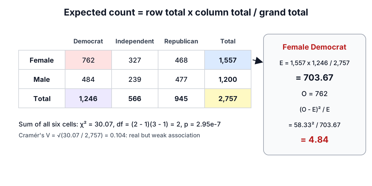
The full set of expected counts is 703.67, 319.65, 533.68 for women and 542.33, 246.35, 411.32 for men. Summing (O - E)² / E over all six cells gives χ² = 30.07.
Degrees of freedom
For an r x c table, df = (r - 1)(c - 1). Here (2 - 1)(3 - 1) = 2. The logic is the same as before: once the row and column totals are fixed, only (r - 1)(c - 1) cells can vary freely. Pearson originally used a different count; Fisher showed in 1922 that this is the correct one.
The right-tail area beyond 30.07 with 2 df is p = 2.95 × 10⁻⁷. Party identification and gender are clearly associated in this sample.
Which cells drive the result?
A significant χ² says the table departs from independence somewhere. To see where, look at residuals. The adjusted standardized residual for a cell is
(O - E) / √(E × (1 - row total / n) × (1 - column total / n))
and under independence each one behaves roughly like a z-score. For the party table:
| Democrat | Independent | Republican | |
|---|---|---|---|
| Female | 4.50 | 0.70 | -5.32 |
| Male | -4.50 | -0.70 | 5.32 |
Women are over-represented among Democrats and under-represented among Republicans, by about 4.5 and 5.3 standard errors; the Independent column is close to what independence predicts. The calculator colours cells beyond ±2.
How strong is the association?
With 2,757 respondents, even a modest association produces a tiny p-value. Cramér's V (Harald Cramér, 1946) rescales χ² to a 0 to 1 effect size:
V = √(χ² / (n × (min(r, c) - 1)))
For the party table, V = √(30.07 / (2,757 × 1)) = 0.104. That is a weak association: real, but gender explains little of party choice. For a 2 x 2 table, V equals the absolute value of the phi coefficient. A common rule of thumb for tables with two rows or two columns, following Cohen, reads 0.1 as small, 0.3 as medium and 0.5 as large.
Small counts and Cochran's rule
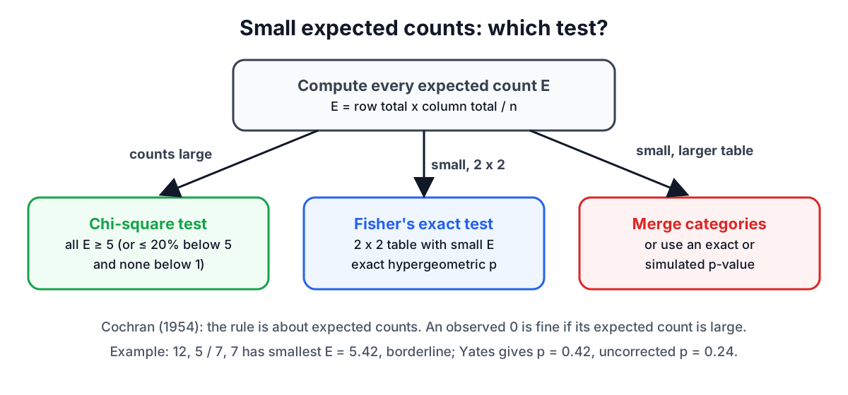
The chi-square distribution is a large-sample approximation. With small expected counts the real distribution of the statistic is lumpy and the p-value can be off. William Cochran's 1954 guidance is still the usual rule: no expected count below 1, and no more than 20% of cells with expected counts below 5. Note that the rule is about expected counts, not observed ones; an observed zero is fine if its expected count is large.
When the rule fails you can:
- merge sparse categories if that makes sense for the question
- collect more data
- use Fisher's exact test for a 2 x 2 table, which computes the p-value from the hypergeometric distribution without any approximation
Yates' continuity correction
For 2 x 2 tables Frank Yates proposed in 1934 subtracting 0.5 from each |O - E| before squaring, to compensate for using a continuous distribution for discrete counts. It always lowers χ² and raises the p-value. Take the small table
| Outcome yes | Outcome no | |
|---|---|---|
| Group A | 12 | 5 |
| Group B | 7 | 7 |
The smallest expected count is 5.42, just above the threshold. Without correction χ² = 1.372 and p = 0.242; with Yates χ² = 0.641 and p = 0.423. The correction nearly halves the statistic.
Statisticians disagree about whether to use it. It tends to make the test conservative, rejecting less often than the nominal α. R's chisq.test and SciPy's chi2_contingency apply it to 2 x 2 tables by default; many textbooks now recommend the uncorrected test for adequate samples and Fisher's exact test for small ones. Whichever you choose, say so, because the difference can decide significance near the line.
Common mistakes
- Using percentages instead of counts. χ² depends on sample size. 60% versus 40% in a sample of 20 is weak evidence; in a sample of 2,000 it is overwhelming. Always enter the raw counts.
- Counting the same subject twice. Each observation must fall in exactly one cell and come from an independent subject. Before-and-after yes/no data on the same people need McNemar's test.
- Testing ordered categories as if unordered. For categories with a natural order, such as age bands or ratings, a trend test is more powerful than the general test of independence.
- Reading association as causation. The test says the variables are related in this sample, not why.
- Reporting only the p-value. Add the degrees of freedom, n and Cramér's V: "χ²(2, N = 2,757) = 30.07, p < 0.001, V = 0.10".
For converting other statistics to p-values, see the p-value guide. For comparing means rather than counts, see the t-test guide.
Frequently asked questions
What is the chi-square formula?
The chi-square statistic, introduced by Karl Pearson in 1900, is χ² = Σ (O - E)² / E. For every category or cell, subtract the expected count E from the observed count O, square the gap and divide by E, then add up the results. Large values mean the counts sit far from what was expected, so the p-value is always the right-tail area.
What if a chi-square expected count is less than 5?
Under Cochran's 1954 rule, no expected count should be below 1 and no more than 20% of cells should have expected counts below 5. The rule is about expected counts, not observed ones. When it fails, merge sparse categories if that makes sense, collect more data, or use Fisher's exact test for a 2 x 2 table.
How do estimated parameters change chi-square degrees of freedom?
In a goodness-of-fit test, each parameter estimated from the same data removes one more degree of freedom, so df = k - 1 - (number of estimated parameters). Testing whether daily defect counts follow a Poisson distribution, for example, means estimating the Poisson mean first and subtracting one more df. Forgetting this makes the chi-square test too lenient.
Can I use percentages in a chi-square test?
No, a chi-square test needs raw counts, not percentages, because χ² depends on sample size. A split of 60% versus 40% in a sample of 20 is weak evidence, while the same split in a sample of 2,000 is overwhelming. Each observation must also fall in exactly one cell and come from an independent subject.
How do I report chi-square test results?
Report the chi-square statistic with its degrees of freedom, the sample size, the p-value and an effect size such as Cramér's V, for example "χ²(2, N = 2,757) = 30.07, p < 0.001, V = 0.10". Reporting only the p-value hides how strong the association is, since large samples produce tiny p-values even for weak associations.
Sources and further reading
- On the criterion that a given system of deviations from the probable in the case of a correlated system of variables is such that it can be reasonably supposed to have arisen from random sampling, Philosophical Magazine. Pearson, 1900.
- On the Interpretation of χ² from Contingency Tables, and the Calculation of P, Journal of the Royal Statistical Society. Fisher, 1922: the (r − 1)(c − 1) degrees of freedom.
- Contingency Tables Involving Small Numbers and the χ² Test, Supplement to the Journal of the Royal Statistical Society. Yates, 1934: the continuity correction.
- Some Methods for Strengthening the Common χ² Tests, Biometrics. Cochran, 1954: the expected-count rule.
- Pearson's Chi-squared Test for Count Data (chisq.test), The R Project. Reference implementation used in the tests.
- Chi-Square Goodness-of-Fit Test (e-Handbook of Statistical Methods), US National Institute of Standards and Technology. The goodness-of-fit form of the test.
- chi2_contingency, SciPy. Applies Yates' correction to 2 x 2 tables by default.
- Agresti, A. (2007). An Introduction to Categorical Data Analysis, 2nd ed. Wiley.
- Cramér, H. (1946). Mathematical Methods of Statistics. Princeton University Press.
Open the Chi-Square Calculator
More Statistics Calculators
Every tool in the Statistics Calculators section, free and in your browser.
- Standard Deviation Calculator
- Mean, Median and Mode Calculator
- Z-Score Calculator
- Confidence Interval Calculator
- Sample Size Calculator
- Permutation and Combination Calculator
- Probability Calculator
- Linear Regression Calculator
- T-Test Calculator
- P-Value Calculator
- Chi-Square Calculator
- Normal Distribution Calculator
- One-Way ANOVA Calculator