
What Is a P-Value? Meaning, Calculation and Misuses
What a p-value measures, how z, t, chi-square and F statistics become p-values, one- versus two-tailed tests, critical values, and the misreadings the ASA warned about.
By Redbison Dev · · Updated · 10 min read

The p-value is the most reported and most misread number in applied statistics. It appears at the end of t-tests, chi-square tests, ANOVA tables and regression output, and it decides which results get called "significant". This guide explains what a p-value measures, how a test statistic becomes one for the four distributions you meet most often, how one- and two-tailed values differ, and which interpretations are simply wrong. The P-Value Calculator does the conversions described here and draws the shaded areas.
The definition, in plain words
Every hypothesis test starts from a null hypothesis, usually "no effect" or "no difference". The test reduces the data to a single number, the test statistic, chosen so that values far from its typical range point away from the null. The p-value is the probability of getting a test statistic at least as extreme as the one you observed, calculated assuming the null hypothesis is true.
So p = 0.03 means: if there were really no effect, data this far from "no effect" would turn up about 3% of the time. Small p-values say the data sit awkwardly with the null hypothesis. They do not say how big the effect is, and they do not give the probability that the null hypothesis is true.
A short history
Karl Pearson computed tail probabilities for his chi-square test in 1900. Ronald Fisher made the p-value central to research practice in Statistical Methods for Research Workers (1925), where he wrote that it was convenient to take 1 in 20, a deviation of about two standard deviations, as a line for judging whether a result deserved a closer look. Jerzy Neyman and Egon Pearson then built a different framework around fixed error rates α and β, with a decision to reject or not. Modern practice is a blend of the two: a p-value from Fisher compared with an α from Neyman and Pearson.
From test statistic to p-value
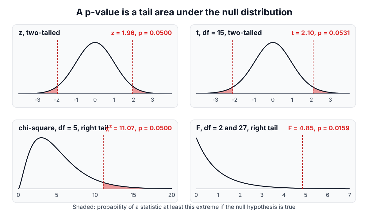
A p-value is an area under the curve of the statistic's distribution when the null hypothesis holds. Which curve depends on the test.
| Statistic | Comes from | Distribution under the null | Usual tail |
|---|---|---|---|
| z | proportions, known σ, large samples | standard normal | two-tailed |
| t | t-tests, regression coefficients | Student t with df | two-tailed |
| χ² | goodness of fit, independence | chi-square with df | right |
| F | ANOVA, regression F, variance ratios | F with df1 and df2 | right |
Worked conversions
- z = 1.96, two-tailed. The area above 1.96 is 0.0249979 and the area below -1.96 is the same, so p = 0.04999579. This is why 1.96 is the 95% multiplier.
- t = 2.1 with 15 degrees of freedom, two-tailed. The right tail is 0.02653, so p = 0.05306. Not quite significant at 5%; with 15 df the statistic needs to reach 2.131.
- χ² = 11.07 with 5 degrees of freedom. The right tail is 0.05001. 11.07 is the printed 5% critical value for 5 df.
- F = 4.846 with 2 and 27 degrees of freedom. The right tail is 0.01591, the p-value of the classic one-way ANOVA on R's PlantGrowth data.
How the areas are computed
None of these curves has an elementary formula for its area, which is why statistics books used to end with pages of tables. The normal tail uses the error function. The Student t and F tails are values of the regularized incomplete beta function: for example, the two-tailed t p-value is I_x(df/2, 1/2) with x = df / (df + t²). The chi-square tail is the regularized upper incomplete gamma function Q(df/2, χ²/2). The calculator evaluates these with continued fractions (the modified Lentz method from Numerical Recipes), computing the upper tail directly rather than as 1 minus the lower tail, so a p-value like 3 × 10⁻⁷ keeps all its digits. Some cases have exact closed forms that make good checks: chi-square with 2 df has tail exp(-x/2), and t with 1 df is the Cauchy distribution, with CDF 1/2 + arctan(t)/π.
One tail or two?
A two-tailed test asks "is there a difference in either direction?" and counts extreme results on both sides. A one-tailed test asks about one direction only and counts one side. For a symmetric statistic like z or t, the one-tailed p-value is half the two-tailed value when the effect goes the predicted way.
That halving is the temptation. A one-tailed test is legitimate only when the direction was fixed before the data were collected and a result in the other direction would lead to the same action as no result at all. Choosing the tail after seeing which way the data point doubles the real false-positive rate. Most journals and regulators expect two-tailed tests unless a one-sided hypothesis was registered in advance.
Chi-square and F statistics are different. They are sums of squares, so any departure from the null makes them larger, whichever direction it goes. Their natural test is right-tailed, and that right tail already includes departures in every direction. A "two-tailed" chi-square or F only makes sense for specialised questions such as testing whether a variance ratio is unusually small as well as unusually large; for those the convention is to double the smaller tail.
p-values and critical values
Before computers, tests were run with critical values: you computed the statistic and compared it with a table value for your α. The p-value approach reports the exact tail area instead. Both give the same decision:
- reject the null at level α exactly when p ≤ α
- equivalently, when the statistic is beyond the critical value
| Test | Statistic | Critical value (α = 0.05) | p-value |
|---|---|---|---|
| z, two-tailed | 1.96 | ±1.95996 | 0.04999 |
| t, df 15, two-tailed | 2.10 | ±2.1314 | 0.0531 |
| χ², df 5 | 11.07 | 11.0705 | 0.0500 |
| F, df 2 and 27 | 4.846 | 3.3541 | 0.0159 |
The p-value carries more information, because it says how far past (or short of) the line the result fell. p = 0.049 and p = 0.051 are, for practical purposes, the same evidence, even though one crosses 0.05 and the other does not.
What a p-value is not
In 2016 the American Statistical Association took an official position on a specific matter of statistical practice for the first time, prompted by widespread misuse of p-values (Wasserstein and Lazar, 2016). Its six principles amount to a list of things a p-value does not do.
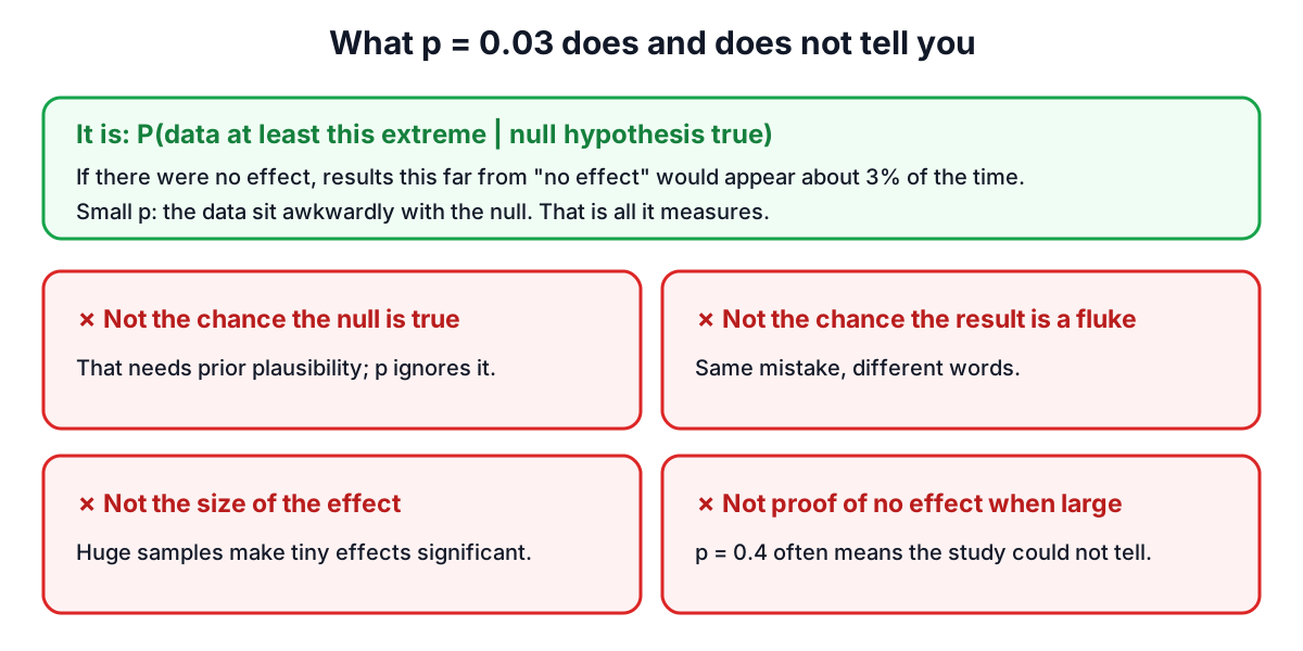
It is not the probability that the null hypothesis is true. p = 0.03 does not mean a 3% chance of no effect. That probability depends on how plausible the effect was before the study, which the p-value ignores. A surprising claim with p = 0.03 remains more likely false than a well-supported one with the same p.
It is not the probability that the result is a fluke. That is the same mistake in different words.
It does not measure the size or importance of an effect. With a million users, a difference of 0.01% in conversion can give p < 0.001. With twelve patients, a large and useful benefit can give p = 0.2. Always report the effect size and its confidence interval.
A large p-value is not evidence of no effect. "Not significant" usually means the study could not tell. A confidence interval that runs from a small harm to a large benefit says exactly that.
A conclusion should not rest on whether p crosses 0.05. The statement asks for full reporting: all the analyses run, the effect sizes, the intervals and the reasoning, not just the significant results.
The multiple testing trap
Each test at α = 0.05 has a 5% false-positive rate when the null is true. Run twenty independent tests on pure noise and you expect one "significant" result; the chance of at least one is 1 - 0.95²⁰ = 64%. Testing many outcomes, many subgroups or many model variants and reporting the best one is how false findings get published. Corrections such as Bonferroni or Holm, used in the ANOVA guide for pairwise comparisons, control the overall error rate.
A practical checklist
- Decide the hypothesis, the test, the tail and α before looking at the data.
- Check the test's assumptions (independence, approximate normality for t and F, enough expected counts for chi-square).
- Report the statistic with its degrees of freedom and the exact p-value: "t(15) = 2.10, p = 0.053", not "n.s.".
- Report the effect size and a confidence interval alongside it.
- Say how many tests you ran, and correct for multiple comparisons where needed.
For the tests themselves, see the guides to the t-test, the chi-square test and linear regression.
Frequently asked questions
Why is 0.05 used as the significance level?
The 0.05 convention traces back to Ronald Fisher's Statistical Methods for Research Workers (1925), where he wrote that it was convenient to take 1 in 20, a deviation of about two standard deviations, as a line for judging whether a result deserved a closer look. It is a convention rather than a law, and p = 0.049 and p = 0.051 are practically the same evidence.
What did the ASA statement on p-values say?
In 2016 the American Statistical Association took an official position on a specific matter of statistical practice for the first time, prompted by widespread misuse of p-values. Its six principles, published by Wasserstein and Lazar, say a p-value is not the probability the null hypothesis is true, does not measure effect size, and should not be the sole basis of a conclusion.
Does a large p-value mean there is no effect?
No. A large p-value usually means the study could not tell whether there is an effect, not that there is none. With twelve patients, a large and useful benefit can give p = 0.2. Report the effect size and its confidence interval: an interval running from a small harm to a large benefit shows that the data are simply inconclusive.
What is the multiple testing problem?
Each test at α = 0.05 has a 5% false-positive rate when the null hypothesis is true, so running many tests makes a spurious "significant" result likely. With twenty independent tests on pure noise, the chance of at least one is 1 − 0.95²⁰ = 64%. Corrections such as Bonferroni or Holm control the overall error rate.
Why is 1.96 used for 95% confidence?
1.96 is the point on the standard normal distribution that leaves 2.5% in each tail. The area above z = 1.96 is 0.0249979, and the same area lies below -1.96, so the two-tailed p-value is 0.04999579. A z statistic beyond ±1.96 is therefore significant at the 5% level, and 1.96 is the multiplier for a 95% interval.
Sources and further reading
- The ASA Statement on p-Values: Context, Process, and Purpose, The American Statistician. Wasserstein and Lazar, 2016.
- Statistical Methods for Research Workers, Classics in the History of Psychology, York University. Fisher, 1925, where the 0.05 convention comes from.
- On the criterion that a given system of deviations from the probable in the case of a correlated system of variables is such that it can be reasonably supposed to have arisen from random sampling, Philosophical Magazine. Pearson, 1900.
- Critical Values of the Student's t Distribution (e-Handbook of Statistical Methods), US National Institute of Standards and Technology. Tables of critical values for comparison.
- Press, W. H. et al. (2007). Numerical Recipes, 3rd ed., sections 6.2 and 6.4 (incomplete gamma and beta functions).
More Statistics Calculators
Every tool in the Statistics Calculators section, free and in your browser.
- Standard Deviation Calculator
- Mean, Median and Mode Calculator
- Z-Score Calculator
- Confidence Interval Calculator
- Sample Size Calculator
- Permutation and Combination Calculator
- Probability Calculator
- Linear Regression Calculator
- T-Test Calculator
- P-Value Calculator
- Chi-Square Calculator
- Normal Distribution Calculator
- One-Way ANOVA Calculator